Our Research

Introduction

There are two position sizes: too little or too much. Too little when it is working and too much when it is not. Of course, our inner idiot compels us to take too little risk when we should be bold and vice versa when we should be prudent.

Position sizing is this critical juncture between financial and emotional capital. Deplete the former and it will take effort to rebuild. It is a complicated problem, but not a complex one. Break the latter and “Game Over”.

On the short side, position sizing is even more critical: failures get bigger and painful, while successes shrink away. Over the years, I have experimented with many position sizing algorithms. Many of them were brilliant, but I would always drift away and abandon each one of them after a while. Then, I realised I looked at the problem from the wrong angle. Convex position sizing is the story of my journey

If You have encountered “fear of pulling the trigger” or if You routinely take too much/too little risk at precisely the wrong time, then this position sizing algorithm might be for You.

 

Part 1: The correct mathematical answer may not be the right one

The first part of the journey was to find out why I consistently drifted from conventional algorithms.

1. Short selling is not a stock picking contest, it is a position sizing exercise

On the short side, the market does not cooperate:

1. Volatility is elevated: that rules out systems like equal weight.
2. Concentrated bets is a bad idea, as their volatility drives the short book and consequently the entire book
3. Short squeezes are frequent: expect all shorts to rally >10% over 5 trading days
4. During bear phases, correlation goes to 1. Expect Longs and Shorts to go against You at once
5. Unprofitable trades balloon rapidly. So, the natural tendency is to be conservative and take small risks.
6. Unlike the long side, there are no 2-3 baggers. Winners shrink and contribute less. So, there is an opposite tendency to oversize positions.

Bottom line: the short side is less a stock picking contest than a position sizing exercise. Winners get smaller and loser get bigger. The difficulty is to size positions so that they contribute when successful, but do not torpedo performance when unsuccessful.

 

2. Two types of algorithms and two types of people

There are two types of position sizing algorithms: aggressive or conservative. Risk seeking systems will have You bet beyond your comfort zone, and sometimes lose more than You should. System failure means cumulative losses have permanently damaged your ability to bounce back.

Conservative systems will have You bet small and earn less than You could. Failure means returns are not attractive enough, and/or period of recovery after a big loss is too long.

There are also two types of people when it comes to risk: risk seeking or risk adverse. Risk seeking people have higher tolerance for the volatility that comes with bold choices. If they go too far, they may no longer have the resources to bounce back.

Risk adverse people accept underwhelming returns in exchange for low volatility. Their downfall is they are sometimes conservative to the point of being risk seeking. Failure does not mean they aim too high and miss their target. Failure means they aim too low and succeed.

 

3. Regime Change, transition and drift

Now, the world is not Manichean. There are times when it is wise to be conservative, settle for a risk adverse system, accept to earn a little less than You could.

There are also times when it pays off to be aggressive, ride a risk seeking system, but potentially lose a lot more than You should.

The problem is that most position sizing algorithms are good at either one or the other. They are not equipped to transition smoothly from equity growth to capital preservation. A core principle is that systems must be followed throughout a cycle in order to achieve predicted results.

 

4. The correct mathematical answer may not be the right one

The problem with many position sizing algorithms is not to find the optimal size that will achieve desired geometric returns. The difficulty is keeping executing through euphoria and depression. Of course, optimal f is the correct position sizing algorithm. The problem is my inner idiot thinks he knows better.

For example, “fear of pulling the trigger” is simply the inner idiot (often referred to as amygdala) saying those bets are too big. This fear gets reinforced after every loss in the thalamus. It eventually gets to the point where the brain overrides the algorithm, but rationalises decisions. Self-deception is insidious, it covers its own tracks.

I did not abandon any of the position sizing all at once. I just gradually drifted away. I failed because my inner idiot constantly second guessed what the algorithms suggested. Discipline is futile. It’s like diet: everyone puts those kilos back on in the end.

I therefore realised that the only way to makes more sense to build a position sizing algorithm that the brain can embrace and then figure out the math.

 

Part 2: Convex position sizing

1. Philosophy of the convex position sizing

Convex position sizing algorithm was conceived backward. Math is subservient to the brain. It may not be the optimal mathematical solution, but it is one my inner idiot will have no problem executing during triumph and disaster.

So, I started out with a list of demands

1. Trade at optimum risk: (accelerator)
   1. Accelerate to maximum risk during run-ups, but
   2. Decelerate quickly as soon as there is a drawdown
2. Absorb volatility: (brakes)
   1. allocate maximum equity, but
   2. reduce risk drastically during severe drawdowns
   3. Avoid whipsaws due to premature re-acceleration
3. Reduce risk for each new re-entry: (trend maturity)
4. Simple input variables (risk appetite)

The best analogy is fuel efficiency. Flooring the accelerator and then slamming the brakes is not a fuel efficient way to drive. These are aggressive systems like Kelly criterion, optimal f and Fixed Ratio Position Sizing (FRPS). Driving like Mrs Daisy is lovely, but not necessarily the most competitive style. These are systems like constant Fixed Fractional Position Sizing (FFPS), equal weight.

Convex position sizing algorithm runs at optimum acceleration. It will take on risk as equity curves rises and reduce as it comes down. It will slam the brakes to avert accidents and then re-accelerate smoothly. Risk Per Trade is the accelerator and Equity would be the brakes.

One of the strengths of the algorithm is smooth transition from risk seeking to risk adverse. The algorithm focuses on drawdowns. As soon as there is a drawdown, risk is reduced. Conventional position sizing algorithms focus on winning streaks and thresholds. They are therefore slow to react.

 

2. Fixed Fractional Position Sizing revisited

Fixed Fractional Position Sizing algorithm basic formula is:

Market Value = Risk Per Trade / Distance to Stop Loss * Equity

Most formulas focus exclusively on Risk Per Trade (RPT). With the notable exception of Market’s Money, few of them consider Equity (capital allocation or surface). The idea became clear to use both sides, one for acceleration, the other for deceleration.

 

3. Convex Risk Per Trade

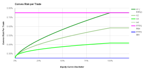
In practice, this is what Risk per trade looks like:

Risk per trade oscillates between a minimum and maximum. Trends mature, so risk per trade is reduced for each re-entry. Convexity comes from the ratio of min/max risk. In this example, min risk is set at -0.25% and max risk at -1%. The bigger the ratio the steeper the acceleration.

How to calculate min and max risk per trade

1. Max Risk per Trade: Risk Appetite / [AVG number of positions * (Long Term Loss Rate + 2 STDEV(Loss Rate)]
   2. Risk appetite: is not a mathematical number. It is the drawdown investors are willing to stomach before redeeming. Whatever You think that number is, divide it by 2. This is a clear case where You do not want to be right !!!
   3. Long Term Loss Rate: ideally, this is the win rate through the entire cycle. When there is not enough sample data, default to a conservative 2/3. That means 2 trades out 3 will fail. 51% Win rate is for fairy tales, and Prince charming is not coming
2. Min Risk per Trade: this is the minimum RPT that would still allow trading during drawdowns
3. Position count: Trends mature. Risk should therefore be reduced after each entry so as to avoid giving back profit on last entries

Risk appetite is one of the two input variable of the entire posSizer algo. Everything else is calculated.

 

4. Drawdon module

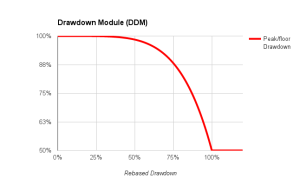
This is the equity allocated to each trade. The objective of this component is to absorb small daily volatility. As a drawdown becomes severe, surface is exponentially reduced so as to collapse residual risk. Note the slope of the curve. Small recovery results in rapid increase of the surface.

Trading floor: this is the second input variable. This is a percentage of equity balance that will be allocated if drawdown exceeds tolerance. A good example here is Millennium partners. After a drawdown of 5%, equity is automatically reduced to 50% of initial capital.

When investors say they can stomach a 20% drawdown, what they mean is they will think about redeeming after a 10% drawdown. So, it is wise to cushion the blow with this drawdown module.

 

Part 3: Convex position sizing in action

This posSizer runs on auto-trade Metatrader MT4. We trade closer to 30 currency pairs, leveraged at 100:1 on 15 minutes periodicity. This is probably as aggressive as it can be.

It feels like being in a driverless Formula 1, without a steering wheel, pedals for accelerator and brakes. Yet, thanks to this algo, there is no need to stay glued to a screen all day. This posSizer provides priceless comfort when most needed. It will smoothly handle trouble: reduce risk, collapse it if necessary and then re-accelerate rapidly.

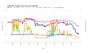
This is what it looks like in practice. Below is a hypothetical equity curve (GS stock price). The real equity curve does not have those big drawdowns, so it is harder to distinguish.

Blue and pink lines are min and max market values per trade (MVPT). Green lines are market values for each position n1 to n4. Orange line is first entry without the drawdown module.

As equity curve rises, MVPT rises in unison. MVPT reacts rapidly to each drawdown but still remains closer to the upper bound until a more pronounced drawdown happens. Risk is reduced for each new tranche.

The drawdown module kicks in during severe drawdowns. This is the difference between the orange and green dotted line. MVPT goes down even further than minimum risk. There are times when even small positions seem too big. This ensures trades go through but at bare minimum risk. This reduces concentration, which in turn sets the stage for a rebound.

One of the problems of FFPS is premature re-acceleration after a drawdown. This leads to whipsaw in sideways markets. This is again a potential reason to drift from suggested positions. After a severe drawdown, the orange line rises faster, while the dotted line adjust re-acceleration to the speed of recovery. For example, the first drop below min risk was followed by a prompt recovery. The second one was more gradual.

 

Conclusion:

Under extreme stress, every degree of freedom, every bit left to interpretation has the potential for costly human error.

Position sizing often overlook the most important component in any trading system: our inner idiot. This algorithm reconciles math and affective neurosciences. It helps us “meet with Triumph and Disaster, and treat those two impostors just the same”, extract from Rudyard Kipling, “If”