Posts

What is the difference between stock trading and gambling in a casino?

MonteCarloAnswer by Laurent Bernut:

I’ll give You the same answer I gave two CIOs of Fidelity. The common point between professional poker players, star fund managers and street hookers is that they go to work: it is not meant to be fun.
Excellent question. Beyond taxes and manufactured negative gain expectancy, there is much market participants could learn from professional gamblers:
  1. Gambler’s serenity prayer: grant me the serenity to accept folding a losing hand, the courage to take calculated risk and the wisdom to know the difference
  2. Cut losses and run winners: in poker, money is made by folding a lot and be aggressive a few times. Successful fund managers spend their time cutting losses. The paradox is that the way to win the war is to accept losing small battles
  3. Position sizing: Black jack is a game where You play against the house. It is manufactured to have You lose. Yet, Edwin Thorpe, whose track record towers Warren Buffet’s, beat the dealer. His method forced casinos to adapt. His secret sauce was position sizing, a fraction of Kelly criterion
  4. Position sizing algorithms: Gambling is a far more mature industry than investing in the sense that a lot of position sizing algorithms used in finance come from game theory. Martingale, reverse-martingale, drawdown/run-up of bankroll, Kelly Criterion
  5. Gambling is boring: hookers, poker players and star managers go to work. It is not meant to be fun. They leave their emotions at the door. Treat gambling and markets as a job so that You can fleece the emotional players
  6. Gamblers have a system: gamblers are not smarter, they have smarter gambling habits. Adherence to a system takes discipline. Reinforced discipline is called habit
  7. Gambling as trading is not a zero sum game: one of the most common myths about the market is the zero sum game. Slippage, commissions erode however slightly the account. Take every trade as if You put a chip on the table
  8. Quantified risk: the notion of calculated risk has unfortunately been perverted by those who do not understand it. Risk is not an abstract dissertation at the end of an investment thesis. Risk is a hard cold probabilistic number
  9. Odds and win rates: one of the fallacies of market participants is the belief they need above 50% win rate to be successful. 2 things here: 1. trading edge or gain expectancy shows that low win rate can be compensated by big payouts. 2, Distributions of P&L of most traders (excluding mean reversion and market making) show aggregate win rates over the cycle of 30-45%. Winners compensate for losers. The important lesson here is that traders walk into a trade expecting it to win, when they should be mentally prepared  for a loss. Pre-packaging grief (see my post: The view from the short-side: how we process emotions and the market signature of the 5 stages of grief Kubler-Ross by Laurent Bernut on Alpha Secure ) . This means that throughout the cycle, styles come and go. Making money means knowing when your style is out of favour and betting small and then when in fvaour take risks. Back to the serenity prayer
Conclusion
Investors usually look down on gamblers. Yet, there is much to learn from gamblers. How come a few of them become successful despite built-in unfavorable odds ?
Beginners in both markets and gambling believe they are on to something when they double down after each loss. They believe that their luck is about to turn, so they use martingale (it comes from the French for winning streak). They just forget two things: dice have no memory so each run is independent from the previous one. More importantly, the maximum expected value is break-even. This means that any outcome other than the best one carries an interesting probabilistic property called “certainty of ruin”.
In other words, there is a reason why casinos have gold, marble columns, master paintings and rookie gamblers go broke…

What is the difference between stock trading and gambling in a casino?

Algorithmic trading: How to get started building an algorithmic trading system?

This is an answer to a question on Quora: Algorithmic trading: How to get started building an algorithmic trading system?

Answer by Laurent Bernut:

If investment is a process, then the logical conclusion is automation.
Algorithms are nothing else than the extreme formalisation of an underlying philosophy.

This is the visual expression of a trading edge
Trading edge = Win% *Avg Win% – Loss% *Avg Loss%
It changed my life and the way I approach the markets. Visualise your distribution, always. It will help You clarify your concepts, shed light on your logical flaws, but first let’s start with philosophy and belief elicitation

1. Why is it important to clarify your beliefs ?
We trade our beliefs. More importantly, we trade our subconscious beliefs. “If You don’t know who you are, markets are an expensive place to find out”, Adam Smith
Many people do not take the time to elicit their beliefs and operate on borrowed beliefs. Unanswered questions and faulty logic is the reason why some systematic traders tweak their system around each drawdown. i used to be like that for many years.
Belief elicitation exercises:

  1. The Work by Byron Katie. After i completed a 2 beliefs a day challenge for 100 days, i could explain my style to any grandmother
  2. 5 why ? Ask yourself a question with “why” and dive deeper
  3. “I am”: beliefs about self are best elicited when we start with this sentence stem
  4. Sentence completion exercises: Nathaniel Branden in his work on self-esteem has pioneered this method. For example, “to me a robust trading is…”

Mindsets: expansive and subtractive or masala smoothie Vs band-aid
There are two types of mindset, and we need both at different times:

  1. Expansive to explore concepts, ideas, tricks etc. Expansive mindset is useful in the early stage of strategy design
  2. Subtractive: to simplify and clarify concepts. Complexity is a form of laziness. Instead of adding yet another redundant factor, try subtracting one or two. Work hard until You find an elegant and simple solution

Systematic traders who fail at being subtractive have a smoothie approach. They throw all kinds of stuff into the optimization blender and waterboard data until it confesses. Bad move: complexity is a form of laziness.
Overly subtractive systematic traders have a band aid mentality. They hard-code everything and then good luck patching
“Essentialist traders” understand that it is a dance between periods of exploration and times of hard core simplification. Simple is not easy
It has taken me 3,873 hours, and i accept it may take a lifetime

2. Exit: start with the end in mind Counter-intuitive truth
The only time when you know if a trade was profitable is after exit, right ?
So, focus on the exit logic first.
In my opinion, the main reason why people fail to automate their strategy is that they focus too  much on entry and not enough on exit.
The quality of your exits shapes your P&L distribution, see chart above
Spend enormous time on stop loss as it affects 4 components of your trading system: Win%, Loss%, Avg Loss%, trading frequency
The quality of your system will be determined by the quality of your stop loss,

3. Money is made in the money management module
Equal weight is a form of laziness. The size of your bets will determine   the shape of your returns. Understand when your strategy does not work and reduce size. Conversely, increase size when it works.
I will write more about position sizing on my website, but there are many resources across the internet

3. Last and very least, Entry
After you have watched a full season of “desperate housewives” or “breaking bad”, had some chocolate, walked the dog, fed the fish, called your mom, then it’s time to think about entry.
Read the above formula, stock picking is not a primary component. One may argue that proper stock picking may increase win%. Maybe, but it is worthless if there is neither proper exit policy, nor money management.
In probabilistic terms, after you have fixed exit, entry becomes a sliding scale probability

4. What to focus on when testing
There is no magical moving average, indicator value. When testing your system, focus on three things:

  1. False positives: they erode performance. Find simple (elegant) ways to reduce them, work on the logic
  2. periods when the strategy does not work: no strategy works all the time. Be prepared for that and prepare contingency plans in advance. Tweaking the system during a drawdown is like learning to swim in a storm
  3. Buying power and money management: this is another counter-intuitive fact. Your system may generate ideas but you do not have the buying power to execute. Please, have a look at the chart above

I build all my strategies from the short side first. The best test of robustness for a strategy is the short side:

  1. Thin volume
  2. brutally volatile: this
  3. shorter cycle: stocks go up the elevator and go out the window
  4. Borrow availability:

Platforms
I started out on WealthLab developer. It has a spectacular position sizing library. This is the only platform that allows portfolio wide backtetsing and optimisation. I test all my concepts on WLD. Highly recommend. It has one drawback, it does not connect position sizer with real live trading.

Amibroker is good too. It has an API that connects to Interactive brokers and a decent poisition sizer.

We program on Metatrader for Forex. Unfortunately, Metatrader has gone down the complexity rabbit hole. there is a vibrant community out there.

MatLab, the expensive weapon of choice for math graduates. No comment…

R: much better cost-performance than Matlab, simply because it is free

Tradestation
Perry Kaufman wrote some good books about TS. There is a vibrant community out there. It is easier than most other platforms

Final advice
If You want to learn to swim, You have to jump in the water. Many novices want to send their billion dollar ideas to some cheap programmers somewhere. It does not work like that. You need to learn the language, the logic.
Brace for a long journey

Algorithmic trading: How to get started building an algorithmic trading system?

Sharpe ratio: the right mathematical answer to the wrong question

Andrew Swanscott runs the podcast Better System Trader. This is great resource: fantastic interviews with real-life practitioners.

http://bettersystemtrader.com/032-laurent-bernut/. I made a statement that attracted a few comments from listeners: Sharpe ratio is the right mathematical answer to the wrong question. Here is the answer as Andrew kindly re-posted on his website.

Sharpe was the right answer

First, let’s start with what Sharpe does well. There are two things it does well:

  1. Cross-asset unified measure: we all know that the most important component in alpha generation is asset allocation. Now, the difficulty is to have a single measure of risk adjusted measure of alpha. This is where Sharpe did the job. It could give a single number across many asset classes: be it fixed income, equities, commodities etc.
  2. Uncertainty: the human brain is hard wired to associate uncertainty with risk. It triggers the amygdala and activates the fight, flight or freeze reflex (see one of my posts about fear and greed). So, Sharpe is a good measure of uncertainty: it quantifies units of uncertainty adjusted performance.

Now, Sharpe ratio, as part of the modern finance package, was invented the same year of the coronation of the Queen of England. It was good, almost revolutionary for its time, since Batista in Cuba was fighting El Che and Fidel. But, like the UN building designed by Brasilian Oscar Niemeyer, it did not age well, and here is why:

Sharpe is not a measure of risk, it is a measure of volatility adjusted performance

Sharpe equates volatility with risk. Risk does not equate volatility and here are a few examples:

  1. Low vol may be extremely risky: LTCM had low vol. In fact, their strategy was to be short gamma. It worked until it did not. Fast forward 2008, vol funds collapsed one after the other. Low vol does not equate risk.  As the great American philosopher Yogi Berra reminded us: “in theory, theory and practice are the same. In practice, they aren’t”. In theory, CDOs and CDs were AAA, low vol high yield products.In practice, they weren’t
  2. CTAs like Ed Seykota, Tom Basso, Bill Dunn, William Eckhardt etc: they have supposedly hopelessly low Sharpe but have clocked >+25% year in year out.

Does it mean that the CTAs have risky strategies ? No, it means they have low semi-volatility adjusted strategies. Semi-vol is just downside volatility.

Volatility means uncertainty, just learn to get comfortable with it

As much as uncertainty is not pleasant and may trigger some reptilian alarms in our brain, we must learn to live with it. It involves mindfulness meditation, strict formalisation of strategies etc. Do not pray for an easy life, pray for the strength to endure a tough one.

Now, what is risk ?

Risk is not a small paragraph at the end of a dissertation called investment thesis. Risk is a number. The only difficulty is to find the adequate formula that goes along. There are two types of strategies: mean reversion or trend following. Please read my posts on the subject.

Risk is not difficult to quantify. It is only difficult to identify. I have come up with the common sense ratio as it recaptures both mean reversion and trend following strategies.

CSR = tail ratio * gain to pain ratio

sense ratio as it recaptures both mean reversion and trend following strategies.

CSR = tail ratio * gain to pain ratio

Please use the trading edge visualiser to find out your personality:

TradingEdgeVisualiser

Conclusion

Bottom line, we have associated risk with volatility. We have come up with a measure of volatility adjusted performance and deem it a risk measure. CSR, on the other hand, is a unified risk measure that can be used across asset classes. It measures risk according to strategy type.

Please subscribe and get some files, material and resources. This is all free so take advantage of it.

The Trading Edge Visualiser User’s Manual

It is impossible to survive in the markets without an edge. Let alone being able to quantify it. How do You know if You even have an edge ?  If You want to articulate a better strategy, You need to 1) understand where your trading edge comes from, 2) quantify it and then 3) gradually improve it. Sharpe, Sortino or Treynor ratios may provide some comfort, but these are just sterile numbers. The smoothie approach of blending indicators and factors into an optimiser has never led to robust breakthroughs. Our brain remembers stories, associates images and concepts. If You can visualise your trading edge, quantify then You will be able to will be able to a better strategy.
The tool I am about to share simply changed my life. It permanently changed the way I approach markets and strategy development. It enabled me to reclassify strategies in two buckets. It then enabled me to understand the pros and cons of each. From there, it showed me the way to improve my trading edge by gradually nudging the distribution. This file is still very much part of my daily development kit. For example, in the summer of 2015 we realised there were many false positives very close to the break even line. We modified just 2 lines in the program, win rate improved by 5% points. This has enabled us to trade higher periodicity while keeping a high win rate.
The Trading Edge Visualiser tool is free. (You may be asked to reconfirm your mail-address, but it is 100% free). It is designed to be simple and intuitive. It will help You
  1. visualise your dominant trading style: mean reversion or trend following
  2. visualise and quantify your trading edge both in aggregate and at individual security level
  3. materially improve your trading edge: we posted some techniques and tips. Try them and see the results for yourself

The trading edge formula

Whatever You believe your trading edge comes from, it can be expressed in this simple formula
      Trading Edge = Win% * Avg Win – Loss% * Avg Loss
The Trading Edge Visualiser is a visual representation of the trading edge. It shows two distributions: absolute P&L and contribution. Contribution is simply P&L divided by Equity.
Green and Orange bars show Buy and Sell (Long & Short) trades. Blue and mauve bars show AVG win, AVG Loss for BUY & SELL. The middle bar is BUY & SELL Trading Edge.

Visual representations of the trading edge of the  styles

Irrespective of instruments traded, there are only two major types of strategies: mean reversion or trend following.

Mean reversion 

Gain Expectancy - Classic Mean reversion
Mean reversion strategies have a Moby Dick shape like distribution:
  1. the hump of the win rate is above the 50% hit ratio line
  2. The long left tail looks like a fin.


 Trend Following

Gain Expectancy - Classic Trend FollowingTrend following strategies have those characteristics
  1. Low win rates: between 30 to 40%. The peak of the loss rate is below the 50% line
  2. Short left tail
  3. Long right tail

 Step 1: Diagnostic

“If You don’t know who You are, the markets are a very expensive place to find out”, Adam Smith
Both Abebe Bikila, the barefoot Ethiopian marathonian, and Hussain Bolt run fast. Yet, marathonians are not good sprinters and vice versa. Similarly, we all have our own trading personality.
The story we tell ourselves about our style and what our trading history shows are two separate things. It is not uncommon to find “value” guys chasing momentum. Neither is it rare to find “momentum” guys doubling down on “cheap” stocks. The first step is to take an honest look at your dominant style. This tool is as honest as the scale in your bathroom.
Process your trading history on the Trading Edge Visualiser. Compare your distribution with the above major dominant styles: mean reversion or trend following.
 

Step 2: Understand and measure the risks associated with your dominant style

Risk is not a dissertation in an investment thesis. Risk is a number. The difficulty is to pick the formula will adequately match the risk associated with your style.
Sharpe, Treynor et al do not measure risk. They measure volatility of returns and naively assimilate volatility with risk. They may have some marginal utility for asset allocation purposes, but certainly not when it comes to quantifying risk.
Relevant risk measures:
  1. Mean reversion: The key risk measure for mean reversion strategies is the Tail Ratio. Tail ratios of 0.3 and below present severe risk of blow-ups. For example, some strategies may clock +0.5% every month, but have a sudden -4% drawdown. This would take 8 months to recover, which is probably beyond the patience threshold of many investors.
  2. Trend following: The key risk measure for trend following strategies is the Gain to Pain Ratio: trend following strategies have low win rates. For example, if You allow each loser to dent your capital by -1%, assuming a 40% win rate, winners will have to average +1.5% just to break even.
Common Sense Ratio
“Common sense is not so common these days”, Voltaire, French freedom fighter
One fine Monday morning at 9 am, I had the honour to meet Jack Schwager. I had just finished his book on risk so I was eager to show him my concocted risk measure. He murmured: “hmm, common sense”. A few days later, I showed it to my boss who cared to elaborate: “hmm, it makes good common sense”. Voila: Common Sense Ratio.
     CSR = Tail Ratio * Gain to Pain Ratio
Lose money 1 < CSR < 1 Make money
CSR is a notable improvement on the tail ratio as it will also capture aggregate profit ratio, or the ability to recover from big losses. It will recapture the inherent cyclicality of trend following strategies via mediocre GPR but high tail ratio.

Step 3: Improve your trading edge

Techniques explained below are designed to nudge the shape of your distribution. Your trading edge is the shape of your distribution. Ideally, You want something that looks like this:

  1. High win rate: not only does it feel better, but it compounds fasterGain Expectancy - Alpha Secure
  2. Long right tail: ride your winners and allow your capital to appreciate
  3. No left tail: cut your losers
  4. Symmetrical distribution on the Long & Short side: identical rules on both sides of the book


Mean reversion

The key to success for mean reversion strategies is to increase the tail ratio. This can be accomplished in two ways:

  1. Stop loss: a strategy without a stop loss is like a car without brakes. As a rule of thumb, a stop loss should not be further away then twice the 90th percentile of your profits. Beyond that limit, the period of recovery may be too long to be commercially acceptable
  2. Elongate your right tail: mean reversion strategies do not allow winners to fully mature. This simple technique can allow winners to develop while preserving profits. Instead of closing the entire position, close no more than 2/3 and place a trailing technical stop loss on the remainder. Do not place a valuation stop loss as it will exceed your comfort zone.
 Moral of the story:
  1. Shops do not restock on products they cannot sell; they mark down the inventory and clear it at a discount. Similarly, do not double down on losers, accept your loss and move on.
  2. “Value” investors usually sell their positions to their “momentum” colleagues, only to sigh in despair when prices subsequently double or triple. Next time, sell them a portion of your holdings and enjoy the ride with them. Worse case scenario, if it does not work, your stop loss will take you out and protect your profit.

Trend Following

Profits look big only to the extent that losses are kept small. So, all You have to do is to manage losses and profits will take care of themselves.
  1. Stop Loss is the second most important variable in your trading system, after the most volatile place on the market, that is the grey box between your left and right earlobes. Stop loss has a direct impact on three out of four components of the trading edge: Win rate, Avg Win, Loss rate. Make a habit of placing your stop loss as your enter your orders
  2. Would You allow tenants to stay rent free in a building You own ? Every time You say yes to a free loader, You say no to a good customer, so make a habit of evicting poor performers
  3. Improve your win rate: assuming average loss stays the same, any improvement in the win rate will have a material impact on the trading edge.
Real life example: i am a short seller. The short side is plagued by periodic tidal waves called short squeezes.  The Trading Edge Visualiser taught me that rather fighting them, it made more sense to use them. I wait for the short squeeze to pass and only after that do I enter at a higher level. Then, as the next short squeeze approaches, I reduce size. This clocks a small win, reduces risk and allows to weather squeezes. Once the squeeze is over, there is a fresh high probability entry point.
This habit of scaling-out and scaling-in tilts the P&L distribution to something like the distribution at the beginner of the paragraph. It combines the high win rate of mean reversion strategies but still has long right tail, short left tail.

File user’s manual

 The Trading Edge Visualiser was built using Metatrader 4 OrderLog. It can be applied to any trading history, provided You load data in the fields coloured in blue and reset the pivot table

 Data load

  • Time and Date: the information is organised in chronological order on the Table sheet
  • Ticket No: this assumes that all trades have a unique identifier
  • Symbol: The table sheet calculates the trading edge of each security in a timely manner
  • Type: Buy/Sell, this allows rapid sort
  • Buy/Sell Lots: this field is useful for multiple entries/exits
  • Profit: this is an absolute USD P&L
  • Contribution: this is a simple P&L / Contribution field. There is no currency conversion, benchmarking or modified-Dietz time-series. Relative performance calculation should take place in this field

 Pivot Table settings

  • ROW fields in Tabular Form: In the PivotTableFields: click on Field Settings: in Layout & Print table: Click on Show items in tabular form
  • ROW Fields SubTotals deactivated: In the PivotTableFields: click on Field Settings: SubTotal & Filters table, Subtotals: click None
  • PivotTable Options Totals Columns deactivated: Right-click anywhere in the PivotTable, go to Totals & Filters, uncheck Show grand totals for columns
  • Column Label: Click on Select All to allow automatic refreshing
 Useful tips:
  1. Run this analysis periodically and keep track of your evolution to receive the full benefits
  2. Truncate data: the current file looks at the entire population. Segment your trading history into blocks when your strategy performs, when it does not.
  3. Comment and annotate entries/exits. You will realise that a bit of finesse on exit will go a long way. It is useful to keep track of exits

Conclusion

People who keep track of their weight are 30% more susceptible to reach their weight loss target. The Trading Edge Visualiser tool will help You understand who You really are. It has the potential to transform your trading game, as it continues to do so for me.

It is 100% free, so download and play with it!

A powerful two step process to deal with the endowment effect: The game of two thirds, or how to deal with free loaders in your portfolio

Would You allow tenants to stay rent-free ?

Would You allow tenants to stay rent-free ?

If You were the owner of an apartment building, would You allow tenants to stay rent-free forever ? You would probably do everything in your power to either collect or evict free loaders. In the investment realm however, one of the main reasons managers fail to accomplish their goals is that they allow free-loaders to stay rent-free in their portfolios. The difficulty then is how to identify and deal with free loaders.

They don’t really stand out enough on an individual basis. Yet, as an aggregate free-loaders put a drag on performance.

  • Endowment effect: once in the portfolio positions are sticky.
  • How to identify and effectively deal with free loaders
  • The 3 main benefits of the game of two thirds
Once upon a time, i used to place thematic small positions across the portfolio like pawns on a chessboard. They were supposedly hedges for China, precious metals, oil, monetary intervention etc. They were all tiny positions that were supposed to kick in if any of these themes were to gain traction. Six months went by and I could not understand why performance was so pedestrian. Meanwhile, none of those stocks had worked. Then, it dawned upon me that even though they were tiny individual positions, they totaled 10% of the portfolio as an aggregate.
The endowment effect (Thaler 1980)
Endowment effect is the hypothesis that people value more what they own than what they could buy. It is hard for positions to dribble their way into our portfolios, but once in they become sticky. It is difficult to get rid of them, even though they do not contribute. Some managers would hold on to losers just because they do not know what to buy next.
Our lives, our desks, our houses are filled with clutter. Unless we actively create and enforce rules to get rid of it, clutter creeps up on us. Our inner saboteur will always find good reasons to hoard junk. To illustrate its potency, let’s look at a simple example: in your wardrobe, isolate the clothes You have not worn for over a year. Think about all the excuses to keep them, but then ask yourself: “If i did not have it, would i buy it now ?” If not, then bye bye, fashion moves on and so should You.
The game of two thirds: A simple two-step process to deal with free loaders
Free loaders neither detract nor contribute enough to be visible. They don’t stand out enough to be dealt with. Since it is not possible to deal with them on the y-axis (price), the solution is to introduce time x-axis. Rationale is simple, if stocks have been there for some time, but still fail to contribute, then their weight should be reduced.
  1. Calculate portfolio turnover, divide it by three: first 1/3. Add 1/3 turnover to the entry date of each position. For example, a stock entered on January 5th and a turnover of 1 would yield a cut-off date of April 5th
  2. Divide performance in 4 quartiles, concentrate on the third quartile: second 1/3. For all stocks in the third quartile past their anniversary date, cut weight in half
 Special mention for long-term winners
Apple (AAPL) or Softbank (9984:JT) are long-term winners. They sometimes go through extended periods of under-performance. Because there is so much embedded profit, it is difficult to realise that they have not contributed for some time. The idea then is to reset contribution on a rolling basis.
The idea then is to apply the same rules as above on a rolling basis. Instead of cutting positions to half, taking a portion the size of the out-performance from the previous haircut. For example, if Apple went up by 10% from previous haircut, then shave 10% off the current size.
The rationale is
  1. if it starts to underperform, it will be dealt with, and this profit taking will have cushioned the blow. This demonstrates stewardship
  2. If it continues to go nowehere, resources are re-allocated to a potentially more productive asset. If non-performance persists over 2/3 of portfolio turnover, then a more drastic reduction is in order
  3. if outperformance resumes, then it will be dealt with
It is important to periodically reset contribution. When stocks have been in the portfolio for a long time and substantially contributed, we become attached. Failure to reset contribution is one of the reasons why some managers escort their positions on the way up and then all the way back down. It doesn’t show until it is too late.
The three benefits of the game of two thirds

The game of two thirds may appear simplistic. It has however powerful psychological implications. It is a simple, powerful and objective way to short-circuit the endowment effect for three reasons:

  1. Simplicity: math is beyond dispute. Simple rules are elegant, easier to implement and harder to challenge
  2. Stewardship: great investors are not smarter, they have smarter trading habits. Getting rid free loaders builds the habit of dealing with difficult stocks
  3. The quality of our excuses determines the quality of our performance: one of the most frequent excuses is “what do i buy next ?” Constant re-examination of positions forces managers into action.
Discussion
Once in a portfolio, positions are often sticky. Asking ourselves “would you buy it again today ?” is too subjective to deal with positions that have overstayed their welcome. Our inner saboteur will find good reasons to procrastinate until the next review. Our natural instinct to hoard junk “endowment effect”. The game of two thirds is an elegant way to identify and deal with free loaders.


The game of two halves: an elegant two-step process designed to cut losers, run winners, while maintaining conviction

In every hospital around the world, there is an unwritten rule: surgeons should not operate on their own children. There is no such thing as professional detachment when it comes to your own child. In the investment realm however, market participants are consistently asked to defend their convictions, but also expected to be surgical about their losers. How can someone maintain enough attachment to weather rough times, but stay detached enough to surgically cut when necessary ?

“Cut your losers, run your winners” is the key to survival in the markets, but no-one tells You how to pick the lock. This is especially difficult if You are a fundamentalist (fundamental analyst/manager/investor/trader). First, there is no price mechanism like a stop loss to tell You it’s time to move on. Second, You don’t want to be perceived as lacking conviction. Third, investors want You to manage risk. No wonder 80% of managers find it difficult to outperform every year.
This is the second article in a series of four about exits and affective neurosciences. Our central premise is that the quality of exits will determine the quality of performance. The purpose of this exercise is to help fundamentalists cut their losers, run their winners, while keeping conviction. It is based on the assumption that they are refractory to the idea of a stop loss policy. It is a simple yet powerful method that is guaranteed to mechanically lift performance.
You do not need to be right 51% in order to make money
One of the classic myth is that “You will make money as long as You are right 51% of the time”. Wrong. You will make money only if You have a trading edge:
                     Trading edge = Average Win% * Win% – |Average Loss%| * Loss %
Let’s take an easy example: if average profit is twice as big as average loss, what would be the break-even hit ratio ?
          0  = 2 * X – 1 *(1-X)
          X     = 1/3
with X = Win% and Loss% = 1- Win%
In a system with a 2/1 profit/loss ratio, you only need to be right 1/3 of the time. In other words, stock pickers who identify 3-5 baggers only need to keep losers small to make formidable gains
In reality, the visual representation of a stock picker’s P&L distribution looks very much like the chart below: a few princes make up for a lot of frogs. . Being right 51% of the time through the entire bull/bear cycle is the unicorn of stock picking. Every strategy experiences a drawdown at some point. Stock pickers make money as long as they stay disciplined and keep their losses small.
 Gain Expectancy - Classic Trend Following
 In order to move to the distribution shown below,  one of two things need to happen:
  1. Either reduce the number of frogs: easier said than done, particularly when strategies stop working at some point through the cycle
  2. or, their impact is reduced: reducing drag will mechanically improve profitability
 Gain Expectancy - Alpha Secure
Predicting tomorrow’s winners is much harder than dealing with today’s losses. The game outlined below is an elegant way to deal with losers. Not only does it mechanically improve the trading edge, it also salvages ego and rewires neural pathways from outcome to process orientation.
The game of 2 halves
The objective is to halve the weight of losers once they detract more than half average contribution. Proceeds are then re-allocated to either fresh ideas or winners. This is a simple two-step process:
  1. Divide all positions between contributors and detractors, calculate average contribution: first half
  2. Reduce weight by half (1/2) for all detractors below -1/2*Average contribution: second half
Example:
Average contribution: +0.5%          Babylon Ltd weight: 4%  Unrealised P&L: -0.4%     Realised P&L: 0%
After weight reduction                      Babylon Ltd weight: 2%   Unrealised P&L: -0.2%     Realised P&L: -0.2%
Now two things will happen: either Babylon Ltd will perish, or it will rise
  1. If Babylon meets a tragically eponymous fate : it would have to drop another -15%, just to reach minus average contribution, or -0.5%. At this point, it will be either it is a screaming Buy or a dog. Either way, it will be an easier decision to make
  2. If Babylon rises: then unrealised profits will compensate for realised losses. One rule of thumb in order to maintain a positive trading edge, do not add to the position until it crosses previous entry price
The additional 2% freed-up can be re-allocated either to winners or fresh ideas. Adding to winners cements conviction. Adding fresh ideas brings fresh blood to the portfolio. Either way, it is more of a good thing.
Special mention for managers who use an equal weight position sizing: Equal weight position has many drawbacks, but it has one benefit in this case. Instead of using contribution (weight * return), a simple distribution of return is sufficient.
The game of two halves has three deep benefits
  1. Trading edge mechanically improves: this is a simple elegant formulation of the first mantra: “cuts your losers and ride your winners”
  2. Good stewardship: managers are often torn between defending their convictions and dealing with problems. If they cut too frequently, they are perceived as lacking conviction, which negatively impacts investors confidence. By selling a portion of the position, they show peers and investors that they both maintain their conviction and deal with problems
  3. Process versus outcome neural pathways re-wiring: funds reach capacity not when they are too big in size, but when inertia sets in. Dealing with losers forces managers into action. This accomplishes three things:
    1. Managers become dispassionate with their problem children: since dealing with them improves stewardship, the stigma of taking a loss disappears. The game is simple enough to be executed even in the darkest
    2. Increased fluidity: since proceeds are re-invested, managers have a direct incentive to look for fresh ideas, or to their existing ones
    3. Process versus outcome mindset: believing that being right about a stock is a matter of profitability is an outcome process. When ideas are profitable, ego gets validation. When (not if) they are unprofitable, ego feels under attack. This invariably leads to defensive, unprofitable and often destructive behaviors. Dealing with losers in an orderly fashion changes focus from outcome to process. Being right is no longer about the outcome but about doing the right thing.
Conclusion
The game of two halves is a key to unlock the “Cut losers and ride winners” fortress. It is an elegant solution to the oldest problem in fundamental investment. It reconciles the demand for conviction with the need for action. The privilege of its (mathematical) simplicity is that it imposes itself even in the darkest times.
More importantly, it changes the definition of being right. It is not a binary outcome on the profitability of individual ideas., It is the observance of a process that will lead to higher aggregate profitability. In the Jungian archetypes, it no longer triggers the orphan (amygdala in the limbic brain, responsible for fight, fight or freeze), but activates the ruler (pre-frontal cortex or thinking brain). In short, the game of two halves reduces stress and improves profitability.

Track record ETF portfolio 2015 – 05 – 15

Nothing speaks louder than a track record. There is no shortage of interesting indicators, strategies, ideas, but in the end, we trust only one thing: track-record. Track record sheds a crude light over two things: robustness of the strategy and quality of execution.
In 2013 and 2014, I wanted to start a hedge fund out of this strategy. We gathered some interest, but we were not able to raise enough assets to make it a viable commercial proposition. Reason was simple: live track-record. The strategy had been running on paper for years, (my bonus was calculated out of it so it was serious), but my employer back then had no interest in seeding a product that would be radically different from their product line-up. Being a sushi chef in a steakhouse does not have a bright long term career prospect.
So, here are three things I have committed to, I will:
  • run this strategy live with real money
  • put 3/4 of my life savings in it
  • publish the track record on our website
Track record for the week-ended May 15th
Attached is a pdf of the track record. The portfolio is still in ramp-up phase. Large positive net exposure is due to the abundance of bullish signals across the investment universe.
Borrow can be thin and fairly expensive for some ETFs. As a results, 3 short candidates were rejected. Borrow ranged from 6% to 9%.
Strategy synopsis
This strategy was developed on the short side, in order to underperform the longest bear market in modern history: Japan equities. This is why it has many counterintuitive features that make sense in aggregate. It relies on three assumptions: persistence of trend, risk management, capital efficiency. If trends persist, then temporary weaknesses/strengths constitute high probability entry points on the Long and Short sides, respectively. It also means that as probabilities recede, risk increases. It is therefore prudent to reduce risk, as trades mature. Capital efficiency simply states that compounded resources put back in circulation should be consistently re-allocated to fresh positions. We assume we cannot predict the future and do not know which trades will be big winners, so we keep on fishing.
The strategy is composed of two modules: entry/exit signals and money management. It takes a bit of grit (> 3,762 hours) to simplify every element to its bare essence. The objective is to continuously invest in successful trends, while reducing risk along the way.
Signal Module
Entry and re-Entry conditions are simple. It is easy to get in, but hard to stay in. Exits, on the other hand, took hundreds of hours for a simple reason: the quality of exits determines the shape of the P&L distribution. Entry is a choice, exit is a necessity. The exit process has been simplified from 9 layers to 3.
  1. Regime definition for all constituents in the universe
    1. Bullish: higher highs & higher lows
    2. Bearish: lower lows & lower highs
  2. Entry: “Buy on Weakness” (Bullish Weakness) and “Short on Strength” (Bearish Strength)
    1. Long: enter the day after a swing low has been recorded && dominant trend is bullish, “Bullish weakness”
    2. Short: enter the day after a swing high has been recorded && dominant trend is bearish, “Bearish Strength”
  3. Exits: There are three types of exits:
    1. Stop Loss: isometric staircase stop loss: all open positions are closed. Stop Loss is calculated as the swing value +/- an allowance for volatility expressed in Average True Range (ATR).
    2. Trend reversal: if a trend reverses from bullish to bearish, all Long open positions are closed. This is the highest possible point at which positions can be logically closed. Symmetrical rules apply on the short side when a trend reverses from bearish to bullish
    3. Risk reduction: every new position carries risk to the equity. So, the priority is o reduce risk. We have developed a proprietary adaptive exit threshold (AET) algorithm that optimizes the quantity to be closed, while reducing risk to near zero level
  4. Re-Entry: re-entries are allowed only after a partial exit has taken place. Re-entries are only possible along the trend
  5. Stock selection and order priority:
    1. Signals: every day, signals on ETFs, Forex and major indices are published on our website. Candidates come exclusively from that list. The exact same information is available to everyone, including myself.
    2. Priority: Candidates are ranked by position size: the bigger, the better. Borrow check happens before position sizing. Thin expensive borrow is an indication of how crowded trades are. All trades with borrowing fee above 5% are rejected. This is the only difference between Longs & Shorts.
Money Management
Money is made in the money management module. Risk is an obsession. Risk is not an abstract debate over a thesis. Risk is a series of numbers, made visual so as to stay painfully compelling at all times. Our basic philosophy is: profits look big only to the extent that losses are kept small. Tomorrow’s reward cannot be predicted, but risk can be managed today. Our proprietary position sizing algorithm responsively manages risk (per trade and in aggregate), exposures, position sizes in real time.
  1. Alpha Secure: This proprietary position sizing algorithm is so impressive that the company was named after it. This is the best tool to weather drawdowns and re-accelerate during winning streaks.
  2. Net exposure:
    1. This is an absolute directional Long and Short model: both sides are expected to generate alpha. Directionality (+/-100%) is only tolerated because of the low correlation between constituents (ETFs). If the universe was composed of stocks within a index, we would run relative series and collapse net exposure to +/- 20%
    2. Net exposure is a direct function of signal generation. For now, the vast majority of signals are bullish. I woke up -100% net short every day for 8 years. So, net exposure will go deeply net negative when needed.
  3. Gross exposure: Gross exposure will be limited to less than 400% so as to avoid margin calls. Gross exposure is a function of market’s money and the Alpha Secure algorithm
  4. Cash deposits: Cash is maintained in various currencies. Forex is another tool in the toolbox to increase equity
Objectives
When managers say “I want to make as much money as possible”, it usually means “I have no risk-control in place”. Expressing objectives in terms of absolute performance percentage points fall into the outcome bias trap. This is a process driven portfolio. Accordingly, objectives are expressed in process metrics. Those are a) reward to risk above 3 for risk management, b) Common Sense Ratio between 1.8 to 2.1 for robustness, 3) trading edge of 0.5 to 1.5 for quality of performance. System will be considered bankrupt if maximum drawdown reaches -20%.
Chart examples:
Charts published every day contain the same information as the ones traded, but presented in a different fashion.

The first chart shows over-imposition of the Buy/Sell strategy over the public chart. They contain rigorously the same information. The only difference is the order logic component, absent in the public display chart, so as not to constitute a Buy/Sell strategy.
  • Stop Loss is the dotted line below each swing Low
  • Numbers preceded by the # sign (for example:#7.6%) are a rudimentary position sizing algorithm that assumes -1% loss to the equity if a position was entered at the Close of the day when the signal happens and stopped at the lower dotted line on the Long side (upper dotted line on the short side)
  • The upper dotted line is a level at which closing half (50%) the position would ensure the trade breaks even thereafter
Black triangles symbolise entries. Stacked black triangles represent single entry but multiple/split exits
Red/Green inverted triangles symbolise exits. Stacked triangles represent final exits. In the example above, the four triangles show the final exit of 4 open positions. Trend reversed from bullish to bearish.
 This is the public version of the same chart. Numbers are rigorously the same. Any smart trader can figure out for herself. In fact, the public version has the advantage of giving free will back to traders. It leads itself to multiple permutations, free from the “mechanical” constraint of a systematic strategy. For example, sideways periods can be used to accumulate stocks, or stay out of the markets.
Below are examples on the short side, with both the “weaponized” and public versions of the same chart. Strategy is symmetrical. It was developed on the short side and then translated to the Long side.
 
The key to being successful on the short side is to take risk off the table. and top-up successful positions. This is exactly what this strategy does.
Charts stripped of Buy/Sell signals lend themselves to multiple combinations and permutations. For example, the three low dotted lines indicated a volatility adjusted inverse head and shoulder pattern: volatility abated and as a result, stop loss moved higher, a movement that preceded a trend reversal.


Regardless of the Asset Class, There Are Only Two Types of Strategies

Finance is one industry where there is no shortage of creativity. There is always a new strategy, investment vehicle, or asset class. This alphabet soup is confusing, particularly when it comes to assessing risk and reward across asset classes. Yet, there is a simple universal way to classify strategies. They fall into two buckets: either mean reversion or trend following. Simply said, the exit policy determines the win rate, which then shapes the return distribution.

Summary

  • A powerful visual representation of style/gain expectancy: Call to Action: our commitment is to help people become better traders. if YOU want to visualise your style, opt-in and we will send YOU a portfolio diagnostic tool for free
  • Regardless of the asset class, there are only two types of strategies: mean reversion or trend following
  • Each strategy type has a specific risk profile, which require different risk metrics. Common Sense Ratio recaptures risk for all strategy types (Read this, it is important)
  • How to increase the win rate, gain expectancy and overall profitability depending on strategy type ?

I. The only two types of strategies: mean reversion or trend following

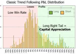
Over the years of patiently testing multiple algorithmic strategies, patterns in the return distribution repeated over and over. It eventually became apparent that strategies fall into two buckets: mean reversion or trend following. Attached are graphical representations of the gain expectancy of mean reversion and trend following strategies. The reason why the same patterns repeat themselves is simple: exit policy.

Market participants tend to treat exit as a single final event. Each trade is a binary event: either it is profitable or not. The accumulation shapes the return distribution. Hit ratio is then determined not by what we enter, but how we exit.

Charts below are return distributions for each strategy type. They are also visual representations of gain expectancy. One image speaks more than a thousand words. This representation changed my life. It permanently altered the way I perceive the markets. The game is about tilting gain expectancy: contain the left tail, moving the peak hit ratio to the right and elongating the right tail. This visual representation is a powerful tool. This is why we want to share it. We are committed to helping people build smarter trading habits. Sign-in to our newsletter (it’s free) and we will send you a portfolio diagnostic tool.

Mean reversion strategies compound small profits

Gain Expectancy - Classic Mean reversion

Death by knock-out: many small profits. a few knock-out blows

Mean reversion strategies compound multiple small profits. They rely on the premise that extremes eventually revert to the mean. They aim ato arbitraging small market inefficiencies. They often have low volatility  consistent performance. They perform well during established markets: bull, bear or sideways. They unfortunately perform poorly during regime changes. They also perform poorly during tail events. The key issue is to contain rare but devastating blow-ups.

 Mean reversion strategies characteristics are (see graphical representation):
  • Moderate to high turnover
  • High win rate: often above 50%. The shorter the duration, the higher the probability of success
  • Consistent small average profits: trades are closed around the mean
  • Low volatility consistent performance
  • Potentially devastating left tail losses: make a little bit of money every day and lose a fortune in one day
  • Long period of recovery after losses:
Examples of mean reversion strategies are
  • Short Gamma: sell OTM options so as to collect pennies in front of a steam roller
  • Pairs trading (non FX): bet on the convergence between two historically correlated securities
  • Value investing: Buy low PBR stocks and “undervalued” assets
  • Counter trend: sell short shooting stars and catch falling knives

Mean reversion strategies post modest but consistent profits. They cater to investors who would look for low volatility returns. Their challenge is the left tail, those infrequent big losses that will take a long time to recoup.

Trend following strategies have a few home-runs 
Gain Expectancy - Classic Trend Following

Death by a thousand cuts: many frogs, a few princes

Trend following strategies rely on the capital appreciation of a few big winners. Whether they follow stories, fundamentals, earnings or price momentum, stock pickers are trend followers. They may fail to appreciate being called trend followers, but their P&L distribution tells a different story.

Trend followers kiss a lot of frogs: they have a low hit ratio, often between 30% and 45%. Performance is cyclical. Styles come in and fall out of favor. Volatility is elevated. Performance can be underwhelming for long periods of time. The key issue is to contain losses during drawdowns.

 Trend following strategies share those common characteristics (see graphical representation):
  • Relatively low turnover
  • Low win rate: 30 to 40%: see chart
  • Big wins and lots of small losses: right tail on chart
  • Relatively higher volatility
  • Pronounced cyclicality: style comes in and goes out of favor
Example of trend following strategies are
  • CTA type systematic trend following,
  • Momentum: earnings momentum, news-flow, price momentum
  • GARP investing: growth at reasonable price
  • Buy & hope
 Trend following strategies post impressive but volatile performance. They can go through long periods of underwhelming performance, which take their toll on the emotional capital of managers. Their main challenge is to keep cumulative losses small. Profits only look big to the extent losses are kept small.
II. How to measure risk for each strategy type
Investors suffer from a “nice guy syndrome”: some young women genuinely say they want to marry a nice guy, but unconsciously react to so-called “bad boys”. Investors genuinely say they want returns, but in reality they do react to drawdowns. More specifically, they are susceptible to drawdowns in three ways:
  1. Magnitude: never lose more than what investors are willing to tolerate
  2. Frequency: lull investors to sleep. Clients will trade performance for low volatility: big money is fixed income, not stocks
  3. Period of recovery: never test the patience of investors.
There are two ways to lose a boxing match: either on points or by knock-out. Mean reversion strategies score until they get knocked out. Trend following strategies lose on points. Risk is not evenly distributed. Therefore, each strategy deserves its own set of risk metrics.
Risk metric for mean reversion strategies: knock-out
Knock-out

Knock-out

Mean reversion strategies have low volatility, consistent performance and high Sharpe ratio. On the surface, they are what investors look for. The problem is mean reverting strategies work well, until they don’t. Big losses are unpredictable. LTCM had a great Sharpe ratio, at least until October 15th, 1987… Risk is in the left tail. The best metric for mean reverting strategies is therefore: tail ratio. Tail ratio measures what happens at the ends of both tails:

Tail ratio  = percentile(returns, 95%) / percentile(returns, 5%)
For example, a ratio of 0.25 means that losses are four times as bad as profits. Turnover then becomes an important variable: the higher the turnover the shorter the period of recovery. The two ways a mean reversion strategy can survive is either by 1) containing the left tail or 2) increasing turnover.
Mean reversion strategies will test investors’ nerves on two things: magnitude of loss and period of recovery. For example,  some strategies such as fundamental pairs trading post constant, reassuring but modest profits like 0.5% a month. Then one day, they post losses of 3 to 5%. They lose in one month the gains of an entire year.
Investors often succumb to the sunk cost fallacy with mean reversion strategies. They believe that big losses are rare and that managers will eventually make them back. This bias ignores probabilities, particularly the theory of runs. It also ignores opportunity costs. The good news is that there is an optimal point below which it makes more sense to redeem than to stick with managers who experienced a severe loss. It is often referred to as optimal stopping. Whilst the formula can be complicated, a simple rule of thumb is to redeem if losses are below 0.4 of turnover.
On the other, trend following strategies have tail ratios ranging from 3 to 10. Winners are much bigger than losers. So, tail ratio is meaningless for trend followers.
Risk metric for trend following strategies: erosion
Trend following strategies have typically low win rates. Risk is therefore not in the tails, but in the aggregates: are a few winners big enough to compensate for the multitude of losers ? Measuring risk then boils down a simple ratio of profits over losses. The risk metric for trend following strategies is therefore:
Gain to Pain Ratio = Sum(profits) / Sum(losses)
Trend following strategies will test investors nerves on frequency of losses and period of recovery. Frequency of losses is another word for volatility. Trend following strategies are volatile, but semi-volatility (downside volatility) is low. They can also post lackluster performance for long periods. For example, mutual funds have built-in cyclicality. Even if they claim to beat the index, mutual funds still lose money during bear markets.
GPR does not apply to mean reversion strategies because blow-ups are unpredictable. GPR can stay high until it is torpedoed by one or two bad losses.
Combined risk metric: Common Sense Ratio
 
 “Common sense is not so common these days”, Voltaire, French freedom fighter
Managers rarely define themselves as adherents of either mean reversion or trend following. Even so, it still would not be easy to assess robustness. Besides, the more risk metrics we use, the more confusing it becomes. For example, some managers have great performance despite a bad Sharpe ratio, so the question is “which matters more in which context?”
Since both metrics outlined above can be expressed in a simple binary ratio, combining them makes sense. When this ratio was first to colleagues and friends in the HF world, comments sounded like “yep, common sense”, hence its imaginative name: Common Sense Ratio
                                                                     Common Sense Ratio = Tail ratio * Gain to Pain Ratio
                                                               Common Sense Ratio = [percentile(returns, 95%) * Sum(profits) ] / [percentile(returns, 5%) * Sum(losses)]
Above 1: make money, below 1: lose moneyCSR is much more powerful than either metric taken individually.
Example 1: GPR = 1.12, TR = 0.25, turnover = 2, CSR =  0.275
Let’s take a classic mean reversion strategy that generates 10% p.a. (GPR = 1.1). It has a moderate turnover of 1.5. Within a 24 months period, it will post a monthly drop of -4%, with a 95% probability. This is 5 times as big as the average profit, and roughly 4 times as bad as right tail profits (TR = 0.25). Common Sense Ratio is CSR = 0.25 *1.1 = 0.275.
On the surface, it may look like a modestly attractive strategy. In reality, the period of recovery combined with magnitude of loss imply that investors will have to be patient. In very simple terms, the CSR shows that returns are not attractive enough to justify investing in such strategies. Try this with a few low volatility strategies. Risk is not where You think it is.
Example 2: GPR = 0.98, TR = 3, turnover = 0.5, CSR = 2.94
Now, let’s take a strategy that loses 2% over a complete cycle (GPR = 0.98). Best winners are 3 times as big as worst losers (TR = 3). Turnover is low 0.5. You may think, why invest in a vehicle that loses money ? It does not make sense. Yet, You are invested in such vehicles: welcome to the average mutual fund. 80% of mutual funds lose roughly 2% to the benchmark. Every now and then, they outperform with a vengeance. The rest of the time they suck air. Morality: over time, mutual funds are poor investment vehicles if You stay invested through the cycle.
III. How to tilt the win rate, gain expectancy and overall profitability depending on your win rate
Gain Expectancy - Alpha Secure
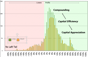
The question boils down to: is it possible to combine the benefits of both strategy types without having the drawbacks of either one ? How can we generate a return distribution that would look like the one on the chart ? (*)
The whole game of investing is about generating a return distribution that would have the following characteristics:
  1. No left tail: small losses like a trend following strategy
  2. Long right tail: big wins like a trend following strategy
  3. High win rate: above 50% win rate like a mean reversion strategy

This type of strategy combines both short term compounding with long-term capital appreciation.

Investors following a mean reversion typically come in early and leave too early. The key is therefore to elongate the right tail. This is done through allowing a remainder to extend beyond the mean with a trailing stop loss.
  1. Set a stop loss (more on this in an upcoming article)
  2. When the trade means reverts, close half the position
  3. Set a trailing stop loss (not based on valuation) and close the trade once the stop loss is penetrated
Bottom line, markets can stay irrational longer than You think. When it stops making sense for You, it may start making sense for someone else. Ride their tail, but protect your downside.
If You are a trend follower, here is a simple game (game of 2 halves) that will mechanically improve your return distribution. We all know that making money is about cutting the losers and riding the winners. Here is an objective way to do it:
  1. Calculate your average contribution, divide it by 2
  2. Reduce by half every losing position below – half average contribution
  3. re-allocate the proceeds to winners
Bottom line, you have reduced losers and increased winners in a simple way (more in an upcoming article)
Conclusion
The  purpose of this article was to introduce a simple yet powerful way to reframe strategies independent of asset class. This enabled us to look at the merits and drawbacks of each type. We then looked at risk metrics that would best recapture their risk profile. We introduced a unified risk metric Common Sense Ratio that works across all asset classes. Finally, we looked at ways to tilt gain expectancy for each strategy type. Last but not least, if You want to know what your trading style, please subscribe and we will send You a diagnostic tool for free.
Preview of the next article:
The next article will deal with investor psychology. Short sellers have a unique perspective on investors psyche. We never sell short against buyers. We observe people who once held a position and are now processing grief. The next article will be about the psychology of grief adapted to the markets.
  1. Market regime: bear markets have several distinctive phases, with a measurable market signature
  2. You will never read an analyst report the same way again. You will learn to read emotions through language and back it up with numbers
  3. You will be better equipped to bottom fish for stocks
(*) : All above return distributions are derived from the same strategy. It has both mean reversion and trend following components. In order to draw a mean reversion strategy, the trend following component was switched off, and vice versa to build a TF distribution. Both components are normally switched on, third distribution